The following table shows what the shapes and ranks are for the various types of
arrays:
Data
Type Shape pX Rank p pX
Scalar No dimension (indicated by a blank line). 0
Vector Number of elements. 1
Matrix Number of rows and the number of columns. 2
N-rank
arrays Each number is the length of a coordinate. N
Empty Arrays
Although most arrays have one or more elements, arrays with no elements also
exist. An array with no elements is called an empty array. Empty arrays are useful
when creating lists (see Catenation in this chapter) or when branching in a user-
defined function (see Chapter 6).
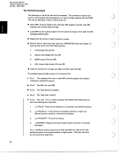
Following are some ways to generate empty arrays:
Assign I 0 to a variable name to generate an empty vector:
%: v 14: c: 'r' C) R
4.. \ 0
I:: \I E: if 'r c1 Ii
An empty array is indicated
4
by a blank display.
6) EZ v E: (1: 'I' IS I?
0
\
The shape of the empty vector
is zero (zero elements).
0 Use a zero length coordinate when generating a multidimensional array:
This matrix has three rows
EM AT R :E X :I. +*3 0 c) 1 0- and no (0) columns.
E.. El 4 'I' li 1: x :I.
4 A blank output display
3 0
~)mmruxi.
0 A function might generate an empty vector as its result; for example, finding the
shape of a scalar:
(3 ' A '
4 A blank output display.
36

CATENATION
(I
You can join together two arrays to make a single array by using the catenation
function. The symbol for this function is the comma. When catenating vectors,
or scalars and vectors, the variables are joined in the order in which they are speci-
fied, as the following examples show:
When catenating two matrices or N-rank arrays, the function can take the form
A,[I]B, where I defines the coordinate that will be expanded when A and B are joined.
If the coordinate is not specified, the last coordinate is used. When A and B are
matrices and [I] is [ 11, the first coordinate (number of rows) is expanded; when [I]
is [2], the last coordinate (number of columns) is expanded. The following examples
show how to catenate matrices:
Graphic Representation
1.0 20 30 11. 22 33 A
B
1.) 0 50 4) 0 414. 55 (5h
A, c2:rs -
10 20 30
40 50 60
A
I 1: j. 3 B
1.0 20 30
I+ 0 5 0 6 0 4
1. :I. 2 2 33 B
1+4 55 66 44 55 66
31